MEGAN software methods

Introduction to MEGAN methods

This tutorial (more like a conversation and notes), will try to introduce to some aspects of the Software MEGAN. I will assume that you are more or less familiar with metagenomics pipelines, and will focus more on how MEGAN does things. The papers and manual that you can check and where I got graphics and information are:

• Huson et al.,MEGAN Community Edition - Interactive exploration and analysis of large-scale microbiome sequencing data, PLoS Computational Biology, 2016, 12 (6): e1004957
• Buchfink et al, Fast and sensitive protein alignment using DIAMOND, Nature Methods, 2015, 12:59-60.
• Huson et al, Integrative analysis of environmental sequences using MEGAN4, Genome Res, 2011, 21:1552-1560.
• Huson et al, MEGAN analysis of metagenomic data, Genome Res, 2007, 17(3):377-86.
• User Manual for MEGAN V6.12.3

There are also useful tutorials:

• Megan Tutorial 2018.key - Algorithms in Bioinformatics
• Taxonomic annotation
• Metagenomics Workshop SciLifeLab Documentation - Read the Docs

Objectives / learning outcomes:

At the end of this tutorial you shoud be able to:

1. Better understand the MEGAN pipeline
2. Underderstand and make use of DIAMOND
3. Know the file formats used in MEGAN
4. Understand the taxonomic assignment by LCA (last common ancestor)
5. Use command line script MEGANIZER to process data
6. Get a gist on the Long Read LCA algorithm: mainly longer contigs
7. Have an idea of the visualization of your data and general analyses

Outline of the tutorial

1. The MEGAN pipeline: a general overview
2. DIAMOND: a lighting fast blast
3. Meganizer: from .daa to MEGAN
4. LCA taxonomic binning
5. MEGANServer: Connecting a server and the app
6. Visualization with MEGAN

The MEGAN pipeline

Overall, MEGAN pipeline can be divided in 4 steps:

1. The input files (already QCed) are analyzed with Diamond (we will get to this in a sec)
2. Diamond (or blast) outputs are converted into MEGAN DAA files
3. Storage in server
4. Interactive inteaction

Basically, you align your reads to a database, bin your reads with annotations, and finally visualize the results. Given that most of your are comfortable with the graphic interface of MEGAN, I will focus on the first three steps.

DIAMOND: a lighting fast blast

DIAMOND stands for Double Index AlignMent Of Next-generation sequencing Data, and you can get it here, and if you haven’t install it now! They report that DIAMOND is ~20,000 times faster than BLASTX. DIAMOND, as MEGAN, are designed for metagenomics, particularly to explore species/OTUs profile, and therefore is usual to align reads to protein databases (hence usage blastx).

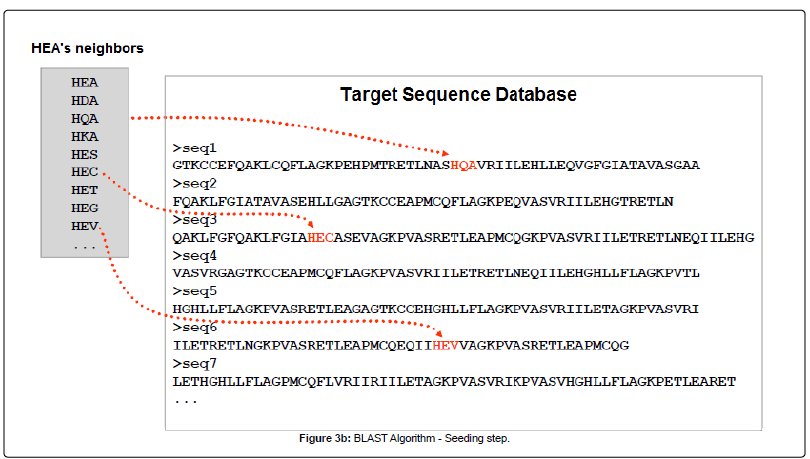
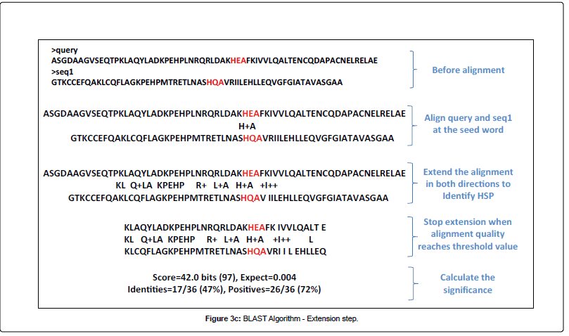
To understand the underlying algorithm of DIAMOND, we need to compare with the traditional blast. Both used the seed and extend strategy (images from Alarfaj et al.):

SEED

EXTEND

However, DIAMOND modifies the seeding in two ways:

1. Reduced alphabet: Their empirical studies allowed them to “re-write” the protein alphabet. This rewrite is done by grouping aminoacids into 11 categories: [KREDQN] [C] [G] [H] [ILV] [M] [F] [Y] [W] [P] [STA].
2. Spaced seeds: Allowing for different “shapes” of seeds and spaces within each seed.
3. Seed index: In short (lots of CS jargon in this), the query is pre-processed and check for common seeds. Each grouped seed is associated with the query names that contains it so that the access during the alignments is faster.
4. Double indexing: Again, lots of CS jargon, but putting symply seeds from subject and query are both index and sorted, making the matching very fast.

More details of the DIAMOND algorithm can be found in this very nice tutorial, and I encourage everybody to read it and bring doubts to other tutorials. From that tutorial:

In summary, here is an outline of the DIAMOND algorithm.

1. Input the list of query sequences $Q$.
2. Translate all queries, extract all spaced seeds and their locations, using a reduced alphabet.
3. Sort them. Call this $S(Q)$.
4. Input the list of reference sequences $R$.
5. Extract all spaced seeds and their locations, using a reduced alphabet. Sort them. Call this $S(R)$.
6. Traverse $S(Q)$. and $S(R)$ simultaneously. For each seed S that occurs both in $S(Q)$ and $S(R)$, consider all pairs of its locations x and y in $Q$ and $R$, respectively: check whether there is a left-most seed match. If this is the case, then attempt to extend the seed match to a significant banded alignment.

Now, let’s compare how DIAMOND does against BLAST. To do so, we need to format the databases both for blastx, and for DIAMOND. I assume you are versed in blast command line tools, and if not, I encourage you to read the tutorial we did a couple of sessions ago. If you are part of the Cristescu Lab, the pre-formated diamond database for nucleotides can be found in our database folder under NCBI. If you are not, please download this file (unfortunately it takes a while and 45Gb). Wether you are part of the CristescuLab or not, format a database (for the Cristescu lab, use a mock fasta file) with the diamond makeblastdb command:

cd PATH/TO/FASTA
diamond makedb --in <FASTA_FILE> -d <NAME_DB>

Replace PATH/TO/FASTA, FASTA_FILE, and NAME_DB with your actual values. In the CristescuLab ~/projects/def-mcristes/Databases/NCBI, I have pre-formatted the full nt database by downloading the fasta file of the entire database (and hence the 45Gb) and executed: zcat nr.gz| diamond makedb -d diamond_nr

Once we have done this, we are ready for the test with this mock fasta file.

Let’s now run a blastx with both BLAST and DIAMOND algorithms (remember to load them or download them): time blastx -db PATH/TO/DATABASE/nr -query /PATH/TO/QUERY/sample.fa -out <OUTFN> -num_threads <CPUS> Just kidding don’t run it… it will take several hours. If you want you can download the results here This one you can run though! Make sure to use a salloc with at least 32 cpus time diamond blastx -d PATH/TO/DATABASE/diamond_nr -q /PATH/TO/QUERY/sample.fa -f 100 --salltitles -o <OUTFN>.daa Or you can just get the result here. Now we have a .daa file (-f is the format, 100 is the binary output format) which basically is the DIAMOND output.

But not everything shines!

In my experience the accuracy drops significantly even with the more sensitive approach. Not great for accurate functional annotation when false positives want to be controlled.

Meganizer: from .daa to MEGAN

After we have a DIAMOND binary output format (MEGAN call it .daa). This file format is DIAMOND proprietary format, but MEGAN supports it. Before we dig into Meganizer, lets take a peak of this file with DIAMOND: diamond view --daa OUTFN.daa | head

The MEGAN user interface uses a different compressed file format called RMA. This is essentially a compressed and comprehensive file that summarizes annotation and classifications to be visualized with the MEGAN GUI. This step takes the information from the alignment to a database (either DIAMOND or BLAST), the taxonomic information, and functional information, and append them in a single file in a relational manner that MEGAN-CE can understand. We can do this either with daa-meganizer or with daa2rma, but we need mapping files between the reference database and the functional annotations. For this example, lets focus in the KEGG annotation, and the mapping file can be downloaded here, and the taxonomic mapping can be found here. These files need to be unzipped. Now let’s check some of the options first: PATH/TO/daa2rma -h

Therefore if we want to include the KEGG annotations we will do: PATH/TO/daa2rma -i OUTFN.daa -o reads.rma -a2t prot_acc2tax-June2018X1.abin -a2kegg acc2kegg-Dec2017X1-ue.abin.zip -fun KEGG

LCA taxonomic binning

The LCA algorithm is explained in this paper. The LCA algorithm has three types: naive, weighted, longReads. The naive algorithm is nice and simple:

Basically, each read is assigned to the lowest common ancestor (LCA) of the set of taxa that had a significant hit in the comparison, and these are binned on that LCA. The taxonomic assignments and the tree above are based exclusively in the NCBI taxonomy (you can add other taxonomies like SILVA). The naive approach bases its assignment solely in the presence/absense of hits between reads.

The weighted LCA has the similar simplicity in mind. However, not only the presence/absense of hits between reads is taken into account, but the number of uniquely aligned hits (kind of similar to OTU abundances).

The LongRead LCA is devised for longer reads and/or contigs. This is the newer development of MEGAN, explained in this paper.

The read is split into intervals (regions) based on the alignment with regions in the reference database. Put in the authors’ words:

a new interval starts wherever some alignment begins or ends.

The significance of the alignment is defined based on the best bitscore: “an alignment is significant if lies within the 10% of the best bit score”. This is a tunable parameter.

MEGANServer: Connecting a Linux server and the app

WHY?? Because the sizes and complexities of metagenomics datasets can be bigger than desktop computers, and to make easier the sharing of data.

With MeganServer one outsources the storage of metagenomic datasets to a different computer and accesses their content via MEGAN.

To set up a server you have to download the standalone version of meganserver, and setup the start script. MeganServer can be then access through the MEGAN GUI.

Visualization with MEGAN

MEGAN have many utilities to visualize your data, here just a few examples (focusing more in non-functional exploration). Most visualization options are regarding the number of reads after filtering.

Basic visualization

By default, MEGAN will display a taxonomic tree (NCBI) and the size of the nodes in the tree is the number of reads in that node.

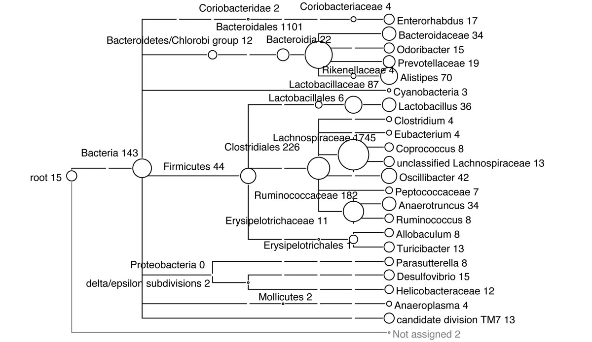
^{https://bmcgenomics.biomedcentral.com/articles/10.1186/1471-2164-12-S3-S17/figures/4}

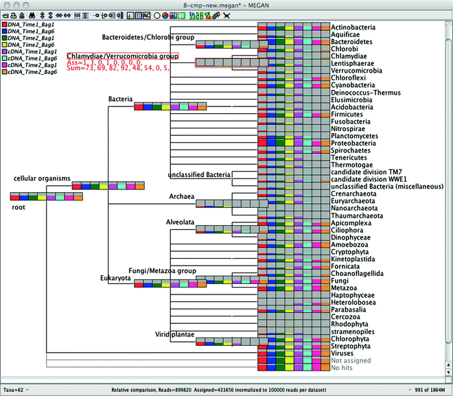
Comparative visualization

In MEGAN one can upload results of multiple datasets and have a comparative view the relative abundance of reads in each sample or group:

^{https://journals.plos.org/ploscompbiol/article?id=10.1371/journal.pcbi.1004957}

Likewise, nodes can be displayed as pie-charts:

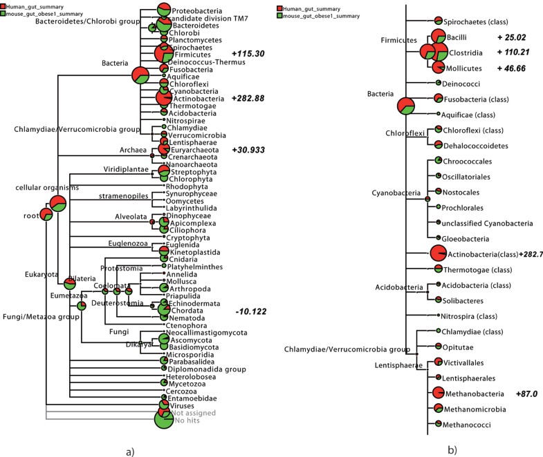
^{https://media.springernature.com/lw785/springer-static/image/art%3A10.1186%2F1471-2105-10-S1-S12/MediaObjects/12859_2009_Article_3195_Fig4_HTML.jpg}

Network visualization/Analyses

MEGAN allows you to represent your data in network from to see the relationships among your samples:

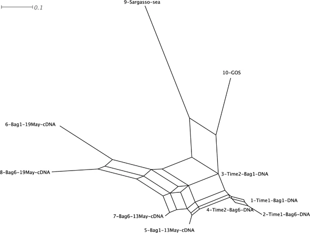
^{https://www.nature.com/articles/ismej201051#Sec3}

Practice time!

Using MEGAN directly is VERY slow if you have not set up the server, so for now we will work with their data-sets to get to know the program: 1) Open from server

2) Connect with Tuebingen server using the guest as both login as password (default)

3) We will work with the daisy dataset. Select all of them.

4) Select all the samples

Now that the server is loaded, let’s explore (This bit is done interactively). 1. What is the most diverse day? 2. What is the best representation for comparative diversity? 3. What does the taxonomy profile tells you? 4. Has the sampling been enough?

Time Permitting: BASTA

Basic Sequence Taxonomy Annotation tool BASTA (Tim Kahlke & Ralph 2018), uses a similar approach to taxonimic binning as MEGAN, the LCA. The pipeline is as follows:

^{Tim Kahlke & Ralph 2018}

Filter weak hits

BASTA has a number of filters available to process your blast output:

1. -e is the evalue threshold which by defaultb is 0.00001
2. -l controls the Alignment length. By default is 100
3. -n Maximum number of hits to use
4. -i Minimum percent identity

Determine hit taxonomy

BASTA matches the each hit with the blast subject taxonomy based on the accession number, thereby circumventing the need for taxids.

Determine Query LCA

After the taxonomy tree has been inferred, each read is map to it and the Last Common Ancestor of the required reads is inferred. Some commands are available to control the LCA algorithm:

1. -m is the minimum number of hits that sequence must have to be assigned an LCA, by default is 3
2. -p Percentage of hits that are used for LCA estimation. Must be between 51-100 (default: 100).

When the p option is different than 100, BASTA will assign the taxonomies where the required percentage of hits are shared.

Output/Visualization

BASTA’s output is a list of taxonomic LCA assignments. When used with th -v option, the most verborse output is given:

### Sequence1
11  Bacteria;Bacteroidetes;
11  Bacteria;Bacteroidetes;Flavobacteriia;
11  Bacteria;Bacteroidetes;Flavobacteriia;Flavobacteriales;
11  Bacteria;Bacteroidetes;Flavobacteriia;Flavobacteriales;Flavobacteriaceae;
6   Bacteria;Bacteroidetes;Flavobacteriia;Flavobacteriales;Flavobacteriaceae;Nonlabens;
1   Bacteria;Bacteroidetes;Flavobacteriia;Flavobacteriales;Flavobacteriaceae;Leeuwenhoekiella;
1   Bacteria;Bacteroidetes;Flavobacteriia;Flavobacteriales;Flavobacteriaceae;Croceibacter;
1   Bacteria;Bacteroidetes;Flavobacteriia;Flavobacteriales;Flavobacteriaceae;Dokdonia;
2   Bacteria;Bacteroidetes;Flavobacteriia;Flavobacteriales;Flavobacteriaceae;Siansivirga;

As per their docs:

In the above example, Sequence1

• had 11 hits in the input blast file
• was assigned Flavobacteriaceae as the LCA (all hits are of this taxon)
• had hits to 5 different genera: Nonlabens (6 hits), Leeuwenhoekiella (1 hit), Croceibacter (1 hit), Dokdonia (1 hit) and Siansivirga (2 hits)

BASTA also ships with extra scripts to plot the results, although it requires KRONA, a hierarchical visualization tool:

I can help you installing BASTA and setting up your first run, but this is outside of this tutorial!!!