Recipe2cuisine

Recipe2cuisine: Part1

In this post I want to share my experience with an Natural Language Processing (NLP) data challenge I tackled at Insight Data Science.

The Goal

Imagibe that you’ve just joined the data team at an online publishing company. One of your verticals is a food publication. A product manager on your team wants to build a feature for this vertical that enables users to query by cuisine, not just by ingredients. Most of your recipes are unlabeled, and it’s infeasible to label them by hand. Luckily, you have a small-ish training set of about 30,000 recipes with labeled cuisines. Design and execute a method to predict the cuisine of a recipe given only its ingredients. For each each major cuisine, what are the driving ingredients that characterize it?

Approach

As always with any data science problem, I have to explore the data, and learn what type of data cleaning/wrangling would be necesary. Our labeled training data looks like this:

[
  {
    "id": 10259,
    "cuisine": "greek",
    "ingredients": [
      "romaine lettuce",
      "black olives",
      "grape tomatoes",
      "garlic",
      "pepper",
      "purple onion",
      "seasoning",
      "garbanzo beans",
      "feta cheese crumbles"
    ]
  },
  {
    "id": 25693,
    "cuisine": "southern_us",
    "ingredients": [
      "plain flour",
      "ground pepper",
      "salt",
      "tomatoes",
      "ground black pepper",
      "thyme",
      "eggs",
      "green tomatoes",
      "yellow corn meal",
      "milk",
      "vegetable oil"
    ]
  }

That is, a json file with a labelled cuisine followed by the ingredients of each recipe. Using pandas and matplotlib, we can plot the number of recipes per cuisine:

%matplotlib inline
import numpy as np
import pandas as pd
from sklearn.feature_extraction.text import TfidfTransformer, CountVectorizer, TfidfVectorizer
import matplotlib.pyplot as plt
from sklearn.model_selection import train_test_split
from nltk.stem import WordNetLemmatizer 
from nltk import word_tokenize  
from sklearn.naive_bayes import MultinomialNB, ComplementNB
from sklearn.pipeline import Pipeline
from sklearn.model_selection import cross_validate
from sklearn import metrics
from sklearn.decomposition import PCA

plt.style.use('ggplot')
filename = '../Challenge_Recipe2Cuisine/recipies.json'
recipes = pd.read_json(filename)
print('Minimum number of ingredients:', recipes.ingredients.apply(lambda x: len(x)).min())
print('Maximum number of ingredients:', recipes.ingredients.apply(lambda x: len(x)).max())
print('Number of cuisines:', recipes.cuisine.unique().shape[0])
recipes.groupby('cuisine').count()['id'].plot(kind='bar') 

Minimum number of ingredients: 1
Maximum number of ingredients: 65
Number of cuisines: 20

<matplotlib.axes._subplots.AxesSubplot at 0x11ca156d0>

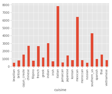
I see that we have a significant class imbalance towards Italian and Mexican cuisine. Also note that 1 ingredient is hardly a recipe, and 65 might be a bit excessive, so let’s plot the distribution of number of ingredients, and let’s print some samples from the extremes:

recipes['n_ingredients'] = recipes.ingredients.apply(lambda x: len(x))
print('Single ingredient\n', recipes[recipes.n_ingredients == 1].head())
print('\nLots of ingredients\n', recipes[recipes.n_ingredients == 65].ingredients.tolist()[0])
recipes.n_ingredients.hist(bins=50)

Single ingredient
          cuisine     id             ingredients  n_ingredients
940     japanese   4734            [sushi rice]              1
2088  vietnamese   7833    [dried rice noodles]              1
6787      indian  36818  [plain low-fat yogurt]              1
7011      indian  19772       [unsalted butter]              1
8181    japanese  16116                  [udon]              1

Lots of ingredients
 ['fettucine', 'fresh marjoram', 'minced garlic', 'olive oil', 'garlic powder', 'large eggs', 'Alfredo sauce', 'vegetable oil', 'cajun seasoning', 'shredded romano cheese', 'basil dried leaves', 'salt', 'cayenne pepper', 'scallions', 'red bell pepper', 'boneless skinless chicken breast halves', 'soba', 'pasta sauce', 'kosher salt', 'milk', 'fresh ginger', 'ground black pepper', 'flour', 'cooked chicken', 'coarse salt', 'lemon', 'diced tomatoes', 'garlic', 'rice vinegar', 'Neufchâtel', 'garlic cloves', 'dried parsley', 'frozen artichoke hearts', 'penne', 'pepper', 'sweet onion', 'part-skim mozzarella cheese', 'parmigiano reggiano cheese', 'basil leaves', 'onion powder', 'red wine vinegar', 'red pepper flakes', 'orzo', 'crushed red pepper', 'all-purpose flour', 'freshly ground pepper', 'sliced mushrooms', 'panko breadcrumbs', 'plum tomatoes', 'fresh basil', 'fresh leav spinach', 'water', 'sun-dried tomatoes', 'ground pepper', 'grated parmesan cheese', 'boneless skinless chicken breasts', 'chicken cutlets', 'butter', 'multi-grain penne pasta', 'extra-virgin olive oil', 'cilantro leaves', 'green pepper', 'shredded mozzarella cheese', 'fresh parsley', 'spaghetti']


<matplotlib.axes._subplots.AxesSubplot at 0x1241415d0>

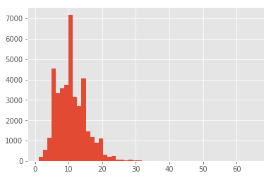
Definitively we have issues with these two classes. Sushi rice, for example, is not a recipe but an ingredient. The second class, contains multiple types of pasta, different sauces, repeated ingredients. This lead me to believe that some recipes have been mistakenly merged, and we need to get rid of such noise. Now focusinng our attention to the histogram, we can see that we have a long tail of low frequency ingredients, most likely composed of those mistakes we already saw. Let’s remove the extreme outside of the 95% confidence through percentiles and reassess:

low = np.quantile(recipes.n_ingredients, 0.05)
high = np.quantile(recipes.n_ingredients, 0.95)
print('Low percentile:', low)
print('High percentile:', high)
sub = recipes[(recipes.n_ingredients >= low) & (recipes.n_ingredients <= high)].copy(deep=True)
max_ing = sub.n_ingredients.max()
min_ing = sub.n_ingredients.min()
print('\nLots of ingredients\n', recipes[recipes.n_ingredients == max_ing].ingredients.tolist()[0])
print('\nFew of ingredients\n', recipes[recipes.n_ingredients == min_ing].ingredients.tolist()[0])
print('\nNumber of recipes after filter:', sub.shape[0])
sub.n_ingredients.hist(bins=15)

Low percentile: 5.0
High percentile: 19.0

Lots of ingredients
 ['black beans', 'olive oil', 'chili powder', 'tortilla chips', 'cheddar cheese', 'store bought low sodium chicken stock', 'chipotle', 'cilantro leaves', 'dried oregano', 'avocado', 'kosher salt', 'ground black pepper', 'garlic', 'sour cream', 'ground chicken', 'cherry tomatoes', 'jalapeno chilies', 'cayenne pepper', 'ground cumin']

Few of ingredients
 ['yellow corn meal', 'boiling water', 'butter', 'fresh parmesan cheese', 'sea salt']

Number of recipes after filter: 36374

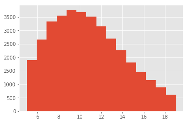
We can see that despite stll having a tail, both the longer and the sorter recipes can be related to actual dishes. In this case it seems that the longer list includes some sort of nachos, and the shorter list, a polenta-like recipe. As you probably already notice, there are a few confounders in the ingredients:

1. Extrenious words such as store bought, and brand names
2. Extra words that might be important for the recipe, but not for classification, such as shredded cheese as opposed to just cheese.

For this post I am going to ignore this and try to classify with the ingredients as they are, and see how we do. In subsequent posts I’ll explain how to deal with such data.

We have, however, seen how imbalance our dataset is. Let’s take a look of what happened after cleaning:

sub.groupby('cuisine').count()['id'].plot(kind='bar') 

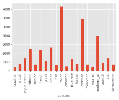
As you can see the imbalance remained. Here I will try first to ignore such an imbalance, but will later revise the model. Since we know that there were mistakes made (e.g. multiple recipes in one), let’s check if there is any mistakes in the ingredients. One way to do this is to plot their lengths and print some of the longer and shorter ones:

sub['min_ingredient_length'] = sub.ingredients.apply(lambda x: min([len(y) for y in x]))
sub['short_ingredient'] = sub.ingredients.apply(lambda x: [y for y in x if len(y) <= min([len(z) for z in x])])
sub['max_ingredient_length'] = sub.ingredients.apply(lambda x: max([len(y) for y in x]))
sub['long_ingredient'] = sub.ingredients.apply(lambda x: [y for y in x if len(y) >= max([len(z) for z in x])])
print('Maximum ingredient lenght', sub.max_ingredient_length.max())
print('Minimum ingredient lenght', sub.min_ingredient_length.min())
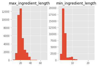
sub.loc[:, ['max_ingredient_length', 'min_ingredient_length']].hist(bins=15)

Maximum ingredient lenght 71
Minimum ingredient lenght 2

print(sub[sub.max_ingredient_length > 65].loc[:, 'long_ingredient'])
print(sub[sub.max_ingredient_length == 71].loc[:, 'long_ingredient'].tolist()[0][0])

283      [bertolli vineyard premium collect marinara wi...
10566    [bertolli vineyard premium collect marinara wi...
14118    [bertolli vineyard premium collect marinara wi...
16156    [bertolli vineyard premium collect marinara wi...
22313    [Pillsbury™ Crescent Recipe Creations® refrige...
26373    [KRAFT Mexican Style Shredded Four Cheese with...
37248    [bertolli vineyard premium collect marinara wi...
Name: long_ingredient, dtype: object
Pillsbury™ Crescent Recipe Creations® refrigerated seamless dough sheet

It seems that even the very long ingredients are not mistakes, but contain many brands. As mentioned before that is a problem for another post. For now, let’s see if we can solved the classification problem linearly. To do this, we can explore our data with PCA, but we first need to tranfor the lists of ingredients into a numerical series. Let’s star with bag of words (BOW) using scikitlearn CountVectorizer. By default, this class will tokenize and pre-process our ingredients by word. As we mentioned before, we do not want that, since it is already tokenized. We therefore need to create a dummy tokenizer and a dummy pre-processing class class, and then create the BOW. However, because eventually we would like to differentiate among classes, we would like to normalized by document. This is done through TF-IDF transformation, since is intended to reflect how important a word is to a document, which will help us also to determine the most representative ingredients in each cuisine:

import re 
class Dummy_Tokenizer(object):
    def __init__(self):
         pass
    def __call__(self, doc):
        # make sure document is a list of lists
        assert isinstance(doc, list)
        return doc

class Dummy_Preprocessor(object):
    def deaccent(self, string):
        #remove accents
        string = string.encode(encoding='ascii',errors='ignore').decode('ascii')
        # also remove things between parenthesis (normally quantities)
        return re.sub("[\(\[].*?[\)\]]", "", string.lower())
        
    def __call__(self, doc):
        assert isinstance(doc, list)
        
        return [self.deaccent(x) for x in doc]
         

vect = CountVectorizer(tokenizer=Dummy_Tokenizer(), preprocessor=Dummy_Preprocessor())
doc = sub.ingredients.tolist()
BOW = vect.fit_transform(doc)
tf_idf = TfidfTransformer().fit_transform(BOW)
# lets make it a dense matrix in pandas (PCA will require this anyhow)
normalized_bow = pd.DataFrame(tf_idf.toarray(), index=sub.cuisine, columns=vect.get_feature_names())
print(normalized_bow.shape)
normalized_bow.head()

(36374, 6475)

	diced tomatoes	frozen chopped spinach	frozen chopped spinach, thawed and squeezed dry	refried beans	sweetened condensed milk	tomato paste	tomato sauce	1% low-fat buttermilk	1% low-fat chocolate milk	1% low-fat cottage cheese	...	yuzukosho	za'atar	zatarains creole seasoning	zatarains jambalaya mix	zest	zesty italian dressing	zinfandel	ziti	zucchini	zucchini blossoms
cuisine
greek	0.0	0.0	0.0	0.0	0.0	0.0	0.0	0.0	0.0	0.0	...	0.0	0.0	0.0	0.0	0.0	0.0	0.0	0.0	0.0	0.0
southern_us	0.0	0.0	0.0	0.0	0.0	0.0	0.0	0.0	0.0	0.0	...	0.0	0.0	0.0	0.0	0.0	0.0	0.0	0.0	0.0	0.0
filipino	0.0	0.0	0.0	0.0	0.0	0.0	0.0	0.0	0.0	0.0	...	0.0	0.0	0.0	0.0	0.0	0.0	0.0	0.0	0.0	0.0
jamaican	0.0	0.0	0.0	0.0	0.0	0.0	0.0	0.0	0.0	0.0	...	0.0	0.0	0.0	0.0	0.0	0.0	0.0	0.0	0.0	0.0
spanish	0.0	0.0	0.0	0.0	0.0	0.0	0.0	0.0	0.0	0.0	...	0.0	0.0	0.0	0.0	0.0	0.0	0.0	0.0	0.0	0.0

5 rows × 6475 columns

With this matrix representation, we can more easily explore how common a given ingredient is. But why would we do that? We want to remove noise from our data, that means ingredients that are too frequent (most cuisines have it) and ones that are only used in a few recipes, can confound the predictions:

ingredients_usage = (normalized_bow > 0).sum(axis=0)
print('Sample of ingredients uses once:\n', ingredients_usage[ingredients_usage == 1].head(), '\n')
print('Sample of ingredients used in at least 10K recipes:\n', ingredients_usage[ingredients_usage > 10000].head(), '\n')
print('Distribution of values:\n', ingredients_usage.describe(), '\n')
low = (ingredients_usage > ingredients_usage.min())
high = (ingredients_usage < ingredients_usage.max())
print('Distribution of values without extremes\n', ingredients_usage[low & high].describe(), '\n')
ingredients_usage.hist(bins=100)

Sample of ingredients uses once:
 2% low fat cheddar chees                   1
2% milk shredded mozzarella cheese         1
33% less sodium cooked deli ham            1
33% less sodium cooked ham                 1
33% less sodium smoked fully cooked ham    1
dtype: int64 

Sample of ingredients used in at least 10K recipes:
 salt    16856
dtype: int64 

Distribution of values:
 count     6475.000000
mean        59.921236
std        364.165886
min          1.000000
25%          1.000000
50%          4.000000
75%         19.000000
max      16856.000000
dtype: float64 

Distribution of values without extremes
 count    4756.000000
mean       77.673675
std       345.920981
min         2.000000
25%         3.000000
50%         9.000000
75%        34.000000
max      7432.000000
dtype: float64 

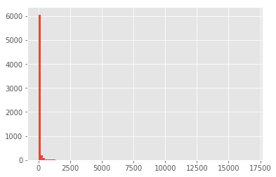
We can see that there are a lot of ingredients that are used only in one recipe, and there are a few used in all recipes (e.g. Salt). For the sake of simplicity, I would remove any ingredient that is use in less than 9 recipes (median of the distribution of values without extremes), and more than 7432 (max value without extremes):

low = (ingredients_usage >= 9)
high = (ingredients_usage <= 7432)
reduced_bow = normalized_bow.loc[:, (low & high)]
print('New shape:', reduced_bow.shape)
ingredients_usage[low & high].hist(bins=100)

New shape: (36374, 2405)

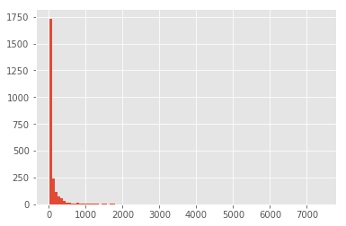
With a somewhat cleaner BOW, we can check how it looks in the first two Principal Components:

cuisines = set(reduced_bow.index)
n_cuisines = len(cuisines)
all_colors = np.linspace(0,len(plt.get_cmap('viridis').colors), n_cuisines, dtype=int)
colors = dict(zip(cuisines, all_colors))
c = [colors[x] for x in reduced_bow.index]   
pca = PCA(n_components=2)
pca_mat = pca.fit_transform(reduced_bow)
plt.scatter(pca_mat[:,0], pca_mat[:,1], c=c, cmap='viridis')

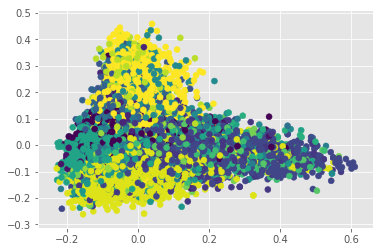
Apparently our problem does not seem to be linear. Let’s confirm this doing an LDA. This step works as a conformation since LDA maximizes the distances between classes, and in doing so, overfits. If a set is not separable by LDA, there is a high likelihood that this problem cannot be solve linearly:

from sklearn.discriminant_analysis import LinearDiscriminantAnalysis as LDA
lda = LDA(n_components=2)
lda_mat = lda.fit_transform(reduced_bow, reduced_bow.index)
plt.scatter(lda_mat[:,0], lda_mat[:,1], c=c, cmap='viridis')

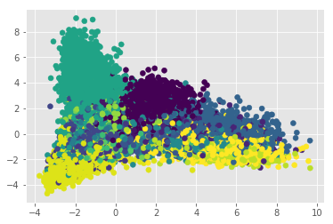
This confirms our suspicions, so we need a more complex model to deal with this classification problem, but before we delve into it, let’s see what are the most representative ingredents per cuisine. We can leverage the TF-IDF normalization since by definition it is “a numerical statistic that is intended to reflect how important a word is to a document in a collection or corpus”:

for name, df in reduced_bow.reset_index().groupby('cuisine'):
    print(name)
    d = df.iloc[:, 1:]
    means = d[d > 0].sum(axis=0).dropna()
    representative = means[means == max(means)].index
    # print the proportion of usage of most representative ingredients in the total of recipes
    print(representative[0], (df.loc[:, representative].astype(bool).sum()/df.shape[0])[0], '\n')

brazilian
onions 0.3477088948787062 

british
milk 0.2623626373626374 

cajun_creole
cajun seasoning 0.19230769230769232 

chinese
soy sauce 0.5137067938021455 

filipino
soy sauce 0.35235378031383735 

french
unsalted butter 0.2300292764533668 

greek
feta cheese crumbles 0.22082585278276481 

indian
garam masala 0.2680334092634776 

irish
butter 0.33766233766233766 

italian
olive oil 0.40968138930671405 

jamaican
ground allspice 0.24008350730688935 

japanese
mirin 0.29049844236760125 

korean
sesame oil 0.4879898862199747 

mexican
jalapeno chilies 0.17570573139435414 

moroccan
ground cumin 0.427972027972028 

russian
sour cream 0.2411504424778761 

southern_us
all-purpose flour 0.2964635063957863 

spanish
olive oil 0.3936750272628135 

thai
fish sauce 0.40211267605633805 

vietnamese
fish sauce 0.46618705035971225 

It makes sense!!. Now we can tackle the classification issue. In this edition of the post I will work with the simplest ML model in my opinion: Naïve Bayes. Since we have multiple classes, let’s try first the Multinomial model. To be able to test the classification we need to split our data into training and testing, and then proceed with the cross-validation:

train, test = train_test_split(reduced_bow, test_size=0.1, stratify=reduced_bow.index)
mnb = MultinomialNB()
mnb_fit = mnb.fit(train, train.index)
pred = mnb.predict(test)
print(metrics.classification_report(test.index.tolist(), pred))

              precision    recall  f1-score   support

   brazilian       1.00      0.11      0.20        37
     british       0.55      0.08      0.14        73
cajun_creole       0.84      0.58      0.69       140
     chinese       0.65      0.92      0.76       252
    filipino       1.00      0.33      0.49        70
      french       0.53      0.41      0.46       239
       greek       0.89      0.30      0.45       111
      indian       0.76      0.92      0.84       263
       irish       0.88      0.11      0.20        62
     italian       0.67      0.90      0.77       731
    jamaican       1.00      0.29      0.45        48
    japanese       0.92      0.59      0.72       128
      korean       1.00      0.43      0.60        79
     mexican       0.85      0.91      0.88       585
    moroccan       0.92      0.46      0.61        72
     russian       1.00      0.02      0.04        45
 southern_us       0.52      0.83      0.64       399
     spanish       1.00      0.12      0.21        92
        thai       0.69      0.78      0.74       142
  vietnamese       1.00      0.10      0.18        70

    accuracy                           0.70      3638
   macro avg       0.83      0.46      0.50      3638
weighted avg       0.75      0.70      0.66      3638

The class imbalance can be affecting the prediction. Let’s try the more robust (in terms of class imbalance) Complement Naive bayes:

mnb = ComplementNB()
mnb_fit = mnb.fit(train, train.index)
pred = mnb.predict(test)
print(metrics.classification_report(test.index, pred))

              precision    recall  f1-score   support

   brazilian       0.89      0.43      0.58        37
     british       0.46      0.15      0.23        73
cajun_creole       0.76      0.62      0.68       140
     chinese       0.67      0.90      0.77       252
    filipino       0.82      0.33      0.47        70
      french       0.61      0.49      0.54       239
       greek       0.77      0.42      0.55       111
      indian       0.73      0.94      0.83       263
       irish       0.57      0.27      0.37        62
     italian       0.76      0.90      0.82       731
    jamaican       0.96      0.52      0.68        48
    japanese       0.85      0.70      0.77       128
      korean       0.97      0.47      0.63        79
     mexican       0.85      0.92      0.88       585
    moroccan       0.83      0.56      0.67        72
     russian       0.75      0.33      0.46        45
 southern_us       0.57      0.80      0.67       399
     spanish       0.70      0.17      0.28        92
        thai       0.65      0.75      0.70       142
  vietnamese       0.57      0.06      0.10        70

    accuracy                           0.73      3638
   macro avg       0.74      0.54      0.58      3638
weighted avg       0.73      0.73      0.70      3638

The improvement is only marginal. Let’s retry doing an under-sampling to make sure is not the class imbalance:

from collections import Counter
def undersample(df):
    gr = df.reset_index().groupby('cuisine')
    c = Counter(df.index)
    smallest = c.most_common()[-1][1]
    under_sampled = pd.concat(sub_df.sample(sub_df.shape[0]).iloc[:smallest, :] for name, sub_df in gr)
    idx = set(df.index).difference(under_sampled.index)
    rest = df.loc[idx, :]
    under_sampled = under_sampled.set_index('cuisine')
    return under_sampled, rest

us, rest = undersample(reduced_bow)
print(us.shape)
us.head()

(7420, 2405)

	tomato paste	tomato sauce	1% low-fat cottage cheese	1% low-fat milk	2% reduced-fat milk	aai	achiote paste	acorn squash	active dry yeast	adobo	...	yellow split peas	yellow squash	yellow summer squash	yoghurt	yolk	yukon gold potatoes	zesty italian dressing	zinfandel	ziti	zucchini
cuisine
brazilian	0.0	0.0	0.0	0.0	0.0	0.0	0.0	0.0	0.0	0.0	...	0.0	0.0	0.0	0.0	0.0	0.0	0.0	0.0	0.0	0.0
brazilian	0.0	0.0	0.0	0.0	0.0	0.0	0.0	0.0	0.0	0.0	...	0.0	0.0	0.0	0.0	0.0	0.0	0.0	0.0	0.0	0.0
brazilian	0.0	0.0	0.0	0.0	0.0	0.0	0.0	0.0	0.0	0.0	...	0.0	0.0	0.0	0.0	0.0	0.0	0.0	0.0	0.0	0.0
brazilian	0.0	0.0	0.0	0.0	0.0	0.0	0.0	0.0	0.0	0.0	...	0.0	0.0	0.0	0.0	0.0	0.0	0.0	0.0	0.0	0.0
brazilian	0.0	0.0	0.0	0.0	0.0	0.0	0.0	0.0	0.0	0.0	...	0.0	0.0	0.0	0.0	0.0	0.0	0.0	0.0	0.0	0.0

5 rows × 2405 columns

train, test = train_test_split(us.iloc[:,1:], test_size=0.1, stratify=us.index)
mnb = ComplementNB()
mnb_fit = mnb.fit(train, train.index)
pred = mnb.predict(test)
print(metrics.classification_report(test.index, pred))

              precision    recall  f1-score   support

   brazilian       0.68      0.57      0.62        37
     british       0.32      0.35      0.33        37
cajun_creole       0.71      0.78      0.74        37
     chinese       0.69      0.73      0.71        37
    filipino       0.68      0.51      0.58        37
      french       0.48      0.41      0.44        37
       greek       0.66      0.84      0.74        37
      indian       0.70      0.84      0.77        37
       irish       0.54      0.41      0.46        37
     italian       0.57      0.62      0.60        37
    jamaican       0.82      0.73      0.77        37
    japanese       0.77      0.61      0.68        38
      korean       0.67      0.81      0.73        37
     mexican       0.67      0.89      0.77        37
    moroccan       0.66      0.89      0.76        37
     russian       0.52      0.46      0.49        37
 southern_us       0.55      0.57      0.56        37
     spanish       0.75      0.41      0.53        37
        thai       0.60      0.71      0.65        38
  vietnamese       0.62      0.49      0.55        37

    accuracy                           0.63       742
   macro avg       0.63      0.63      0.62       742
weighted avg       0.63      0.63      0.62       742

We can see now more balance scores, although there is plenty of room for improvement an overall f1-score of 65 is not the sexiest f1-score, but will do for this post. Plase keep an eye open for follow-up posts.

I’ll be happy to get your comments and suggestions!!